ABSTRACT
Probabilistic segmentation is an integration of image segmentation and classification, originally developed for multi-spectral images of agricultural areas. Here, this method provides improved classification, by considering spatial coherence within agricultural fields, in addition to spectral crop characteristics. The method is based on Bayesian classification, where the posterior probability for each class (given the feature vector of a pixel) is calculated from the probability density of that feature vector within the class, and the prior probability for the class within an image segment. An iterative procedure estimates those class prior probabilities within arbitrary image segments, as the relative contributions of the classes to the segment's area. To avoid problems of over-segmentation and under-segmentation the algorithm is applied in a segmentation pyramid: a collection of segmentations with varying coarseness. In a final step, complete area coverage is built from different pyramid levels using class purity criteria.
In this study probability density estimation is extended to hyper-spectral imagery by applying a k-nearest neighbor algorithm. The advantage is that this is a non-parametric method, without necessity to assume a distribution and to estimate its parameters (which might be too many in the hyper-spectral case). With the richness of spectral information in hyper-spectral data, application of the method to natural vegetation mapping becomes feasible. Although such vegetation occurs in a less orderly manner than agricultural crops, it also does not grow completely randomly. Therefore, considering spatial coherence, provided by probabilistic segmentation improves classification results also in this case. A vegetation type classification is shown from a coastal area on the island Schiermonnikoog in the Waddensea, to the North of the Netherlands.
1 INTRODUCTION
The Dutch Ministry of Transport, Public Works and Water Management is, amongst other tasks, responsible for protection against floods. It is involved in the control and management of a major part of Dutch coastal zones, and, as a derived responsibility, in the protection of ecosystems in those zones. Monitoring and mapping of natural vegetation, therefore, belongs to the tasks of the Survey Department of the Ministry. Remote sensing is the preferred surveying technique, since it has the potential to frequently observe large areas, allowing for timely discovery of changes (degradations) that might occur.
Image classification is the technique for (semi-) automatic mapping of land cover, in this case natural vegetation, on the basis of remote sensing imagery. Traditionally, classification attempts to assign one class (from a user-defined set of land cover classes) to each image pixel, on the basis of the spectral information (an array of remotely-sensed reflection measurements in different wavelengths) contained in that pixel. It is implicitly assumed that there is a label in the set that adequately characterises the entire pixel, meaning that (a) no other classes occur in the area than those in the set, and (b) the pixel is entirely, or at least predominantly, covered by a single class. If the first of these assumptions is not guaranteed, the classifier should be able to assign the label unknown to pixels that do not seem to belong to any class in the set. Failure of the second assumption, i.e. the presence of mixed pixels, is a well-known classification problem. A solution might be sought in classifiers that are able to recognise the ambiguity and attach some form of confidence level to each labelled pixel.
[Fisher] distinguishes between several types of mixed pixel: caused by boundaries between homogeneous areas, by intergrades (gradual transitions between classes), and by objects that can be considered line-features or point-features in the given image resolution (Fig. 1)
It is important to distinguish the problem of mixed pixels from the phenomenon of spectral overlap between classes. The latter occurs when two pixels that belong to different classes cannot be distinguished spectrally (i.e. contain the same reflection measurements). This does not necessarily mean that those classes cannot be spectrally distinguished at all, but rather that both classes show spectral variation to an extent that the two collections of reflection measurements overlap. Whereas the mixed-pixel problem is related to spatial resolution, spectral overlap has a relation with spectral resolution. Both problems (mixed pixels and spectral overlap) are very influential during classification for mapping of natural vegetation.
Therefore specialized methodologies are necessary. In this study, the usefulness of Probabilistic Segmentation [Gorte 98] is investigated. After this introduction, Section 2 further elaborates on image classification for natural vegetation mapping. Section 3 introduces soft classification, distinguishing between fuzzy and sub-pixel approaches and their application fields. Section 4 is the core of the paper, describing probabilistic segmentation and its adaptation to hyper-spectral image classification methods. Section 5 describes classification of coastal natural vegetation in a case study. Section 6 gives conclusions and recommendations.
2 VEGETATION TYPE CLASSIFICATION
In an early but crucial stage during classification the set of classes has to be defined. An obvious choice is to use plant species as the classes. A drawback is that the number of species in a given area may be quite large, and exceed the number of classes that can be reasonably handled by a classifier. More importantly, most of the pixels in the image will become mixed, since many species rarely cover large contiguous areas, but are always accompanied by other species. Related to this is that the required scale level for mapping individual species is much larger (more detailed) than the image resolution allows for.
Alternatively, vegetation types can be used instead of species. A vegetation type is an agglomeration of certain species in more or less typical proportions, which is characteristic for a significant number of places in the entire area.
The advantage is that properly chosen vegetation types can be mapped on a much smaller (coarser) scale than species, such that the resulting map gives a much better overview of the area, and can be used at a more appropriate management level - anyhow, management and maintenance of naturally vegetated coastal zones does not concern individual plants. In image classification terms it means that the probability for a pixel to have contain a single type is much larger than the probability that it has contains a single species - there are much fewer mixed pixels when types are used.
The relationship between vegetation types and plant species is many-to-many. As said, a type contains several species; moreover, a the same species can participate in several types. Nevertheless, the number of vegetation types, needed for a useful in a certain area is usually smaller than the number of species, which is favourable for classification purposes. At the other hand, vegetation types are expected to be spectrally less distinct than individual species, and even less homogeneous. However, this cannot be used as an argument in favour of using species as the classes, if single-species pixels hardly occur.
3 SOFT, FUZZY AND SUB-PIXEL CLASSIFICATION
Classification as described above is commonly called crisp, meaning that a single class label is assigned to each image pixel. Ambiguous situations, originating from mixed pixels or from spectral overlap, pose a problem for crisp classifiers.
[Eastman] reviews soft classification approaches, which allow for assignment of more than one class label to an image pixel. Within soft classification, a distinction can be made between fuzzy and sub-pixel classification, depending on which of the two ambiguity problems it intends to solve:
- In order to handle the uncertainty originating from spectral overlap, fuzzy classification identifies the possible classes and assigns membership values. Depending on the underlying classification method, membership values can be, for example, Bayesian probabilities, Dempster-Shafer beliefs neural network activation levels or fuzzy set possibilities.
- In order to solve the mixed-pixel problem, sub-pixel classification identifies the participating classes and estimates their proportions.
Fuzzy classification methods are preferred in case of a lack of spectral image resolution, while spatial resolution is considered sufficient. An example might be classification of agricultural areas in SPOT imagery to estimate crop acreages. Sub-pixel classification, on the other hand, seems feasible when spatial resolution is the bottleneck, as it is often the case in NOAA (AVHRR) imagery, but also in e.g. geological applications of hyper-spectral imagery, when sparsely occurring minerals are to be identified [Neville 03].
In many cases, the distinction between fuzzy and sub-pixel classification, both from theoretical and practical (i.e. application) point of view is not as clear as in the above discussion. [Eastman] reminds that a calibration procedure may be required to translate membership values to proportions [Foody, 2000], although some techniques, particularly those based on Bayesian probabilistic, assume a direct linear relationship between posterior probabilities and class area proportions. This is also the case in Probabilistic Segmentation, a soft classification method, which in this study has been adapted to vegetation classification in hyper-spectral imagery.
4 PROBABILISTIC SEGEMENTATION
Probabilistic Segmentation [Gorte 98] is an image analysis method consisting of a combination of image segmentation and soft classification. The classification is fuzzy in the sense that in each pixel Bayesian posterior probabilities are used as class memberships (see section 4.1 below). Subsequently, these probabilities are used to establish class area proportions. Like in sub-pixel classification, it is recognised that one pixel can contribute to several classes; however, the purpose is to compute the proportions within mapping units (image regions showing thematic homogeneity in terms of the map user), rather than within individual pixels (section 4.2)
The mapping units, in turn, are formed by image segmentation using a quadtree-based region-growing algorithm. It generates a hierarchy (pyramid) of segmentations at different levels of coarseness (section 4.3). A feedback loop selects complete area coverage from the various levels on the basis of class-purity criteria (section 4.4).
Probabilistic segmentation simultaneously addresses the problems of spectral overlap and of mixed pixels, particularly the intergrade case (Fig. 1b), which is quite typical for natural vegetation.
4.1 Bayesian classification
Given a pixel with feature vector x (consisting of reflection measurements in a number of spectral wavelength bands) Bayesian classifiers calculate for each class Ci (i = 1 ... N) the posterior probability P(Ci | x) that the pixel belongs to that class, according to the formula of Bayes:
The right hand side consists of:
- P(x | Ci) : the conditional probability to find feature vector x within class Ci . This probability is estimated by analysing samples of Ci , pixels that the user designated as belonging to class Ci during the training stage of the classification. The collection of estimates of this probability for each feature vector x determines the probably density function of a class.
- P(Ci) : the prior probability for class Ci , which is the relative area that Ci covers in the image, or in a designated region of the image (containing the pixel under consideration)
- P(x) : unconditional feature density, the probability that feature vector x occurs in the image (or in the above-mentioned region) - P(x) is often not considered since it is the same for all classes; when the possibility of an unknown class is not considered, P(x) can be replaced by a normalisation factor, since at the end the posterior probabilities (one for each class) add up to 1.
Probability density estimation
The probability density function for class Ci is a function of x, denoting the probability that that feature vector occurs in that class. It is estimate on the basis of the training samples for Ci , where it is a problem that there are many more possibilities for x than there are training samples. A common solution is to assume a parametric distribution (for example a multi-variate normal distribution) and to estimate the parameters (mean vector and covariance matrix). Drawbacks are that this assumption may be not valid, and (especially important with hyper-spectral imagery, say with d bands) that the parameters are a mean vector with d elements, and a covariance matrix of d * (d+1) / 2 elements, requiring a large number of samples for a reliable estimate.
Therefore, in this study non-parametric estimation was used, based on an (approximate) k-Nearest Neighbour searching algorithm called ANN, developed by [Arya and Mount 93].
The ANN program documentation [ANN 03] contains:
ANN is a library written in the C++ programming language to support both exact and approximate nearest neighbour searching in spaces of various dimensions. [...] ANN is also a test bed containing programs and procedures for generating data sets, collecting and analysing statistics on the performance of nearest neighbour algorithms and data structures, and visualizing the geometric structure of these data structures.
In the nearest neighbour problem a set P of data points in d-dimensional space is given. These points are pre-processed into a data structure, so that given any query point q, the nearest (or generally k nearest) points of P to q can be reported efficiently. ANN is designed for data sets that are small enough that the search structure can be stored in main memory (in contrast to approaches from databases that assume that the data resides in secondary storage). The distance between two points can be defined in many ways. ANN assumes that distances are measured using any class of distance functions called Minkowski metrics. These include the well known Euclidean distance, Manhattan distance, and max distance.
In the above description, the set P of data points is the collection of d-dimenstional feature vectors of all training samples (for all classes together). The feature vector x of a pixel to be classified is used as a query point (in the above description). ANN returns then the k nearest (i.e. spectrally most similar) training samples, after which it is possible to distribute these according to their classes, which yields a sequence of numbers ki , i = 1 ... N.
To transfer these neighbours-per-class counts ki into class probability densities P(x | Ci), the number of samples Si per class has to be taken into account as well. Otherwise, the probability densities would be biased towards classes with more training samples. It can be shown that unbiased estimates are obtained by taking P(x | Ci) proportional to ki / Si [Gorte 98].
4.2 Local prior probabilities
Prior probabilities of classes to occur in a pixel can either concern the entire image, or be confined to an image region (that contains the pixel), for example as obtained by image segmentation. Such local prior probabilities are expected to contribute to more refined classification results. As an example, knowing that a certain grass species occupies 80% of the dunes in a coastal zone area, is inside these dunes much more relevant than knowing that this grass species occupies 4% of the entire image (in which the dunes cover only a small portion).
Bayes's formula is used to derive posterior probabilities from probability densities and prior probabilities (replacing the unconditional feature density P(x) by a normalizing factor).
[Gorte and Stein 98] have shown that (local) prior probabilities, taken as relative area proportions, can be derived from posterior probabilities, by using the posterior probability P(Ci | x) as the proportion of the pixel that is covered by Ci. This is were the transition between membership values and sub-pixel proportions, as mentioned in section 3, takes place. Although this may be a doubtful step within a single pixel, it is justifiable within a region. For example, if in a region of 100 pixels the posterior probability for grass is 0.3, this may be interpreted as an expectation that 30 of those pixels are grass. Then, on average each pixel gives a contribution of 0.3 to the total grass area within the region.
Now that posterior probabilities and prior probabilities mutually depend on each other, an iterative procedure is required to compute both of them simultaneously. This procedure has been proven to converge into sensible estimates.
Summarizing, given a arbitrary segmentation of the image (preferably into relevant mapping units), we are able to calculate within each segment the class proportions, in an iterative procedure. Note that in many regions only a single class may be present. By using the class proportions as prior probabilities, posterior probabilities are computed for each class in each pixel during the same procedure, as in fuzzy classification. The input for the iterative procedure consists of the probability densities, as computed from the training samples using a k-Nearest Neighbor method. An implicit assumption is that probability densities within a class are global, independent of image segments or mapping units.
4.3 Image segmentation
The regions in which local prior probabilities (class area proportions) are calculated, may be obtained by any image segmentation method. Also manual segmentation by visual image interpretation might be feasible, since humans are very skilled in identifying relevant units in aerial images. Subsequently, the task of assigning class labels by crisp or soft classification may still be automated, especially when using hyper-spectral imagery, which cannot be interpreted easily by humans.
In this study, however, a quadtree-based region-growing image segmentation method is applied, which recursively merges pixels into segments and segments into larger segments, while obeying spectral homogeneity criteria. These state that 2 neighbouring segments will be merged if:
1. the spectral distance between them is smaller than a threshold T1 .
2. the elements of the covariance matrix in the merged segment do not exceed a threshold T2 .
Experiments have shown that these two thresholds can be safely replaced by a single threshold T, with T1 = 3 * T and T2 = T2 .
Choosing larger values for T leads to coarser segmentations, with an increased risk of over-segmentation: the creation regions that are too large from a user's perspective, such that relevant information is lost. Conversely, smaller values for T give finer segmentations, that are prone to under-segmentation, the creation of irrelevant details. Unfortunately an optimal value does not exist. Intermediate values will show over-segmentation at some places and under-segmentation at others.
Therefore, we apply an ascending sequence of threshold values and store all the resulting segmentations in a segmentation pyramid, having a very coarse segmentation (in the extreme case: a single segment covering the entire image) at the top, increasingly fine segmentations when going downwards, and finally a very fine segmentation (in the extreme case consisting of 1 pixel per segment) at the bottom. Since the segmentations are constructed by region merging, the pyramid is built up in a bottom-up manner.
4.4 Segment selection
In a final processing stage, local prior probabilities are calculated in all segments of all segmentation pyramid levels. It may be expected that in higher pyramid levels, where segments are (too) large, almost every segment will show a mixture of many classes (with corresponding prior probabilities). This reveils that those segments might have to be further subdivided. Near the bottom of the pyramid, however, segments are probably pure (consisting of only one class with prior probability 1), but the number of segments is too large to be mapped. Classifying all these small segments would be equivalent to a pixel-by-pixel classification. The hypothesis of probabilistic segmentation is now that for each position in the area an "optimal" pyramid level can be found, in the sense that when going further up the purity of the segment deteriorates (the number of contributing classes increases), and when going further down the purity does not improve (the number of classes does not decrease). Of course, this optimal level is not the same over the entire image, since a single optimal segmentation threshold does not exist.
In very many places this strategy will just select a pure segment at the highest level possible, and "crisply" assign a label to the segment. But in other places a mixed segment will be selected, when further down in the pyramid no purer segments are found either. After that, the choice is still open whether to assign more than one label in a fuzzy fashion to the entire segment, or to crisply classify the individual pixels in the segment according to maximum posterior probability.
5 CASE STUDY
The imagery used was collected with the HyMap (hyper-spectral mapping) system, which is an airborne whiskbroom scanner. The swath width is determined by the opening angle of the scanner (60�), in which 512 pixels are recorded. The scanner distinguishes 128 spectral bands of 10-20 nm width, in the wavelength interval between 400 nm and 2500 nm, and with 16 bit radiometric resolution. The spatial resolution depends on the flying height and speed, and on the integration time of the sensor.
The images were recorded above a salt-marsh area on the island of Schiermonnikoog, one of the Wadden-islands to the North of the Netherlands, on May 27th, 1999. Four strips were flown in East-West direction. The flying height of 1650 m resulted in a strip width of almost 2 km and a pixel size of approximately 3.5 x 3.5 m.
The German Aerospace centre (DLR) determined the relative and absolute orientations of the strips and established the geometric corrections (geo-referencing) of the images on the basis of differential GPS measurements and orientation observations in the plane. The resulting geometric precision of the imagery was not revealed, but the standard deviation is certainly larger than one pixel. As a consequence, the training stage of the classification, on the basis of detailed field measurements, became extremely difficult.
For training the classifier and validating the classification results 384 field-recordings were available, which were split in equal numbers of training and validation samples. During the research, classification schemes were applied at different hierarchical levers (table 1). These schemes are not based on spectral characteristics of the classes, but rather on user requirements concerning the classification result. Therefore, classes show spectral overlap even in hyper-spectral images.
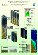
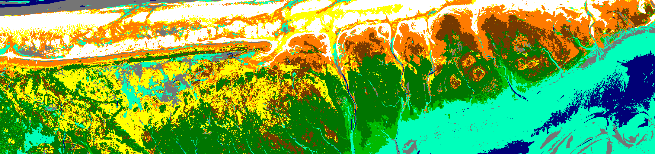
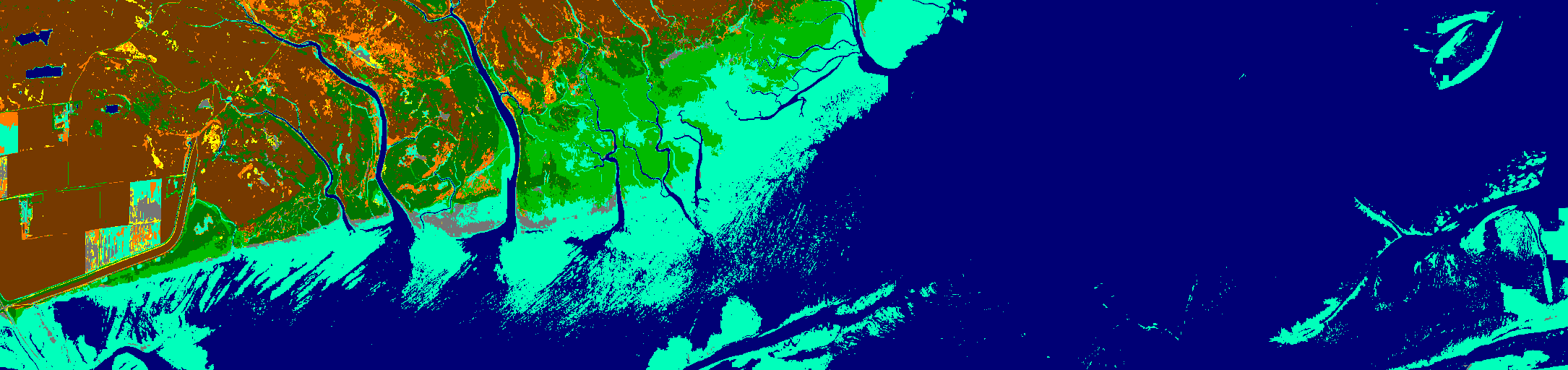
For all three aggregation levels the complete probabilistic segmentation procedure was executed. To give an impression, Figure 2 shows a the result of a level 1 classification in 2 out of 4 strips.
Comparing the classification result with the test samples yielded estimates of an overall classification accuracy of 67.4 %, whereas a crisp pixel-by-pixel k-Nearest Neighbour classifier yields an accuracy of 61.9%. Given the small number of training samples, standard maximum likelihood classification can only be applied to images containing a smaller number of selected spectral bands, which leads to even smaller accuracies.
6 CONCLUSION
We have shown the adaptation of probabilistic segmentation to hyper-spectral imagery and its applicability for natural-vegetation mapping using vegetation types, rather than species. The approach is fully justifiable from a theoretical point of view, and is justified in practice by an increase in overall classification accuracy. It must be noted, however, that the accuracy figures are severely distorted by problems during collection of training and evaluation samples. Firstly, it was hard to find "pure" samples at any aggregation level. Second, the samples were difficult to locate exactly in the images, given the geometric image correction with more than one pixel standard deviation. Finally, class definitions and aggregation levels were established, and training samples collected, without having a particular classification method in mind. Most likely, a more directed approach could improve the results. Of course, also the results of a crisp classifier would benefit from these improvements.
Nevertheless we consider this application of the method successful, since it (slightly) improves classification, and reveals classified regions that can be readily used as mapping units.
Table 1. Class definitions at different aggregation levels.
| Level 1 |
Level 2 |
Level 3 |
1  Bare soil and sparse veg. Bare soil and sparse veg. |
1 Bare soil and sparse veg. |
1 Bare soil and sparse veg. |
2  Pioneer salt-marsh Pioneer salt-marsh |
2 Salicornia-Suaeda veg. |
2 Salicornia (high cover) |
| 3 Salicornia-Suaeda |
| 4 Suaeda-Limonium |
3  Low marsh Low marsh |
3 Puccinellia vegetation |
5 Puccinellia-Salicornia-Limonium |
| 6 Puccinellia-Glaux |
| 4 Limonium vegetation |
7 Limonium |
| 5 Halimione vegetation |
8 Halimione |
4  Medium high marsh Medium high marsh |
6 Juncus-ger. vegetation |
9 Juncus-Suaeda-Limonium |
| 10 Juncus-Festuca |
| 7 Festuca vegetation |
11 Festuca |
| 12 Artemisia |
| 8 Juncus-mar. vegetation |
13 Juncus mar. |
| 9 Elymus vegetation |
14 Elymus |
5  High marsh High marsh |
10 Potentilla vegetation |
15 Potentilla-Juncus |
| 16 Agrostis-Potentilla |
| 11 Sagina vegetation |
17 Sagina-Armeria |
6  Dune-marsh transition Dune-marsh transition |
12 Dune-marsh transition |
18 Dune-marsh transition |
7  Dune Dune |
13 Dune |
19 Dune |
8  Beach Beach |
14 Beach |
20 Beach |
9  Water Water |
15 Water |
21 Water |
REFERENCES
[ANN 03] http://www.cs.umd.edu/~mount/ANN/ - Website for downloading and documentation of ANN software (visited 28 June 2003).
[Arya and Mount 93] S. Arya and D.M. Mount, "Approximate nearest neighbor searching", in Proc. 4th Ann. ACM-SIAM Symposium on Discrete Algorithms (SODA'93), 1993, pp. 271-280.
[Eastman 02] J.R. Eastman and R.M. Laney. "Bayesian Soft Classification for Sub-Pixel Analysis: A Critical Evaluation". Photogrammetric Engineering & Remote Sensing, 68, nr. 11 (2002), pp. 1149-1154.
[Fisher 97] P. Fisher, "The pixel: a snare and a delusion". International Journal of Remote Sensing, volume 18, nr. 3 (1997), pp. 679-685.
[Gorte and Stein 98] B. Gorte and A. Stein, Bayesian Classification and Class Area Estimation of Satellite Images Using Stratification, Trans.GeoRS (36), No. 3, May 1998, pp. 803-812.
[Gorte 98] B.G.H. Gorte, Probabilistic segmentation of remotely sensed images. Ph.D. thesis, Wageningen University, 1998.
[Neville 03] R.A. Neville, J. Lévesque, K. Staenz, C. Nadeau, P. Hauff and G.A. Borstad. Spectral unmixing of hyperspectral imagery for mineral exploration: comparison of results from SFSI and AVIRIS, Can. J. Remote Sensing, Vol. 29, No. 1, pp. 99-110, 2003.
[Wang 90] F. Wang, "Fuzzy supervised classification of remote sensing images". IEEE Transactions on Geoscience and Remote Sensing, volume 28, nr. 2 (1990), pp. 194-201.